Edge computing IoT battery life optimization — Practical Guide

Introduction

Problem statement: In production IoT fleets, battery capacity is the binding constraint on feature set, deployment cadence, and total cost of ownership.

Promise: This article gives engineers a practical, production-tested set of strategies for extending IoT device battery life, with architecture patterns, code snippets, diagnostics, and a decision checklist you can apply today.

Failure scenario (example): A remote environmental sensor running TinyML inference wakes every 10 seconds to evaluate an event. Network uplinks are frequent and unbatched. Battery drains in weeks instead of months. The device logs show high radio-on time, repeated cold-start inference, and no effective sleep scheduling. The result is costly field maintenance and missed business SLAs.

News hook: With TinyML tooling and Cortex‑M TinyML patterns now shipping in volume in 2025–26, the question shifts from “can we run ML at the edge?” to “how do we do it for years on battery?” The patterns below are what senior embedded and ML engineers use to close that last-mile gap.

Executive Summary

TL;DR: Use local, event-driven edge inference, aggressive radio batching, duty-cycled sensors and CPUs, and hardware-assisted wake to reduce active time; combine software techniques (quantization, early-exit models) with runtime policies (adaptive sampling, sleep scheduling) to extend battery life by 3–10x depending on workload.

• Run inference where it reduces network transmissions — but only when model cost < saved comms energy.
• Reduce active time: duty-cycle sensors & MCU, use wake-on-motion/wake-on-radio, and schedule radios for batched uploads.
• TinyML power optimization: favor int8 quantization, pruning, and model early-exit; keep RAM usage low to avoid additional DRAM power.
• Sleep scheduling algorithms: choose deterministic schedules for predictable events and adaptive schedules (reinforcement or heuristic-based) for variable environments.
• Measure the dominant cost (sensing vs compute vs comms) and optimize that first; in >80% of outdoor sensors, radio comms dominate energy use.
• Build observability: sample p95/p99 active-time, radio-on-time, and inference latency to correlate battery drain with behavior.

Three direct Q→A pairs (one-liners)

• Q: When should I run inference on-device? A: Run local inference when it prevents a radio transmission more often than the cost of the inference itself (compute cost < comms cost amortized over avoided transmissions).
• Q: Which TinyML optimizations give the largest battery wins? A: Quantization to int8, pruning to reduce MACs, and early-exit models — in that order for most Cortex-M deployments.
• Q: How to estimate battery-life gain quickly? A: Build an energy model: measure energy per transmission, per inference, and per second in active/sleep; battery-life scales roughly as BatteryCapacity / (p_active * E_active + p_sleep * E_sleep).

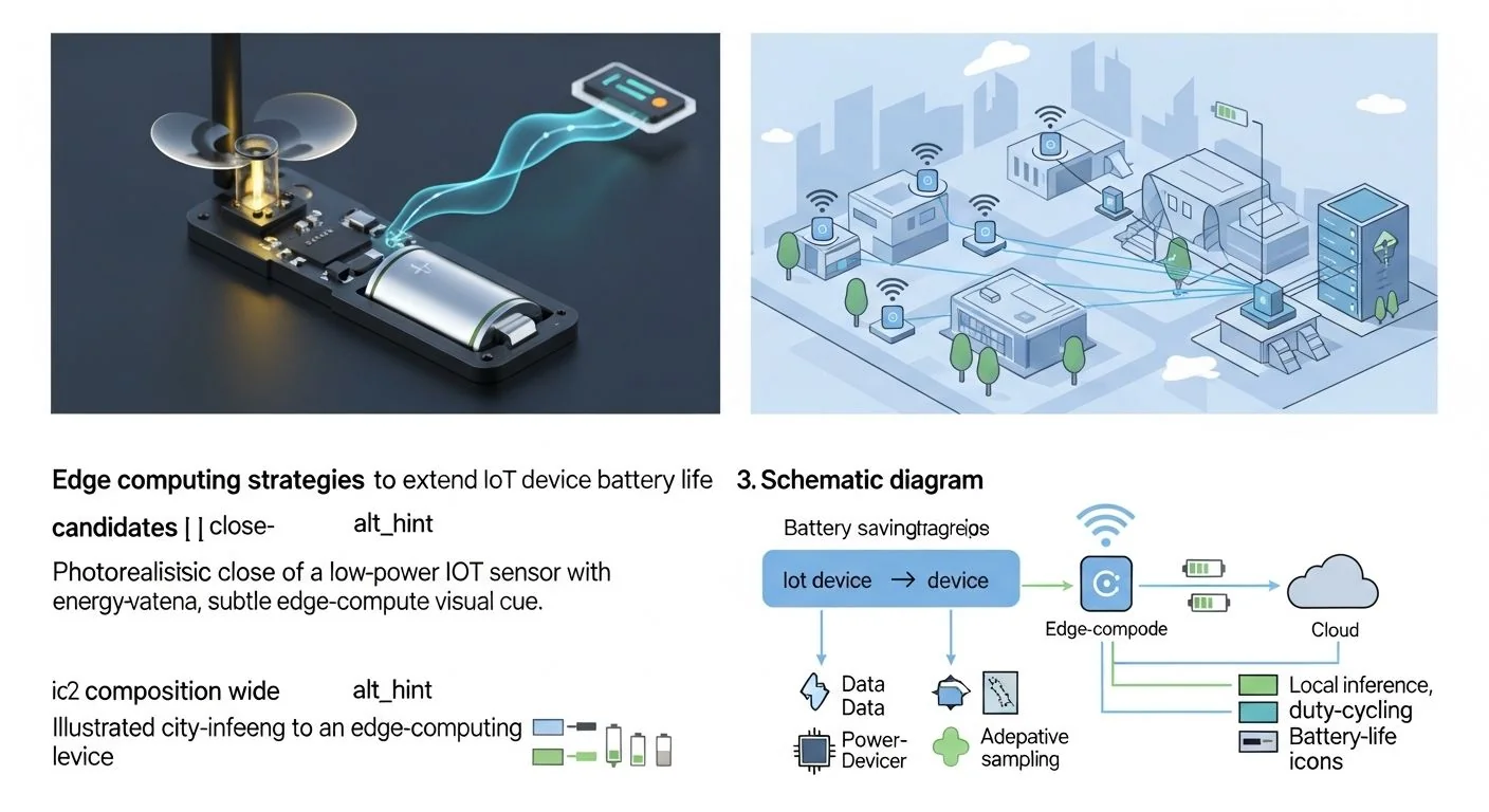
How Edge computing strategies to extend IoT device battery life Works Under the Hood

Edge strategies target the three dominant energy sinks on an IoT node: sensing, compute, and communications. The operating principle is simple: minimize active time and the number of expensive radio transmissions by moving inexpensive computations to the node and using hierarchical decision logic and TinyML patterns.

Architecture components and interactions (textual diagram):

1. Sensor layer: event-driven peripherals (accelerometer, microphone, low-power ADC) with built-in wake-on-motion or programmable thresholds.
2. Wake layer: hardware interrupt + low-power timer that transitions the MCU from deep sleep to an active context.
3. Edge inference layer: compact TinyML model executing in a microcontroller runtime (TF Lite Micro or fixed-point inference kernel) to classify or detect events locally.
4. Decision & aggregation layer: local logic or lightweight rules engine that decides whether to send a report; aggregates events for batching.
5. Comms layer: low-power wireless (LoRaWAN, NB-IoT, BLE, or Wi‑Fi Synchronous Low-Power modes) with duty-cycled radio use and scheduled uplinks.
6. Management & OTA layer: secure update, remote telemetry, and energy-aware fleet policies delivered via a low-frequency control channel.

Algorithms & protocols that reduce energy:

• Event-driven sampling: sensor interrupts replace polling loops (saves CPU cycles and energy).
• Duty-cycling & batching: group sensor readings and network transmissions to amortize radio wake cost.
• Local filtering/classification: suppress transmissions for negative or common cases using TinyML models.
• Model early exit & cascade inference: run a small classifier first, only invoking larger models when needed.
• Adaptive sampling: increase sampling when activity is detected, reduce it otherwise (hysteresis to avoid thrash).

Implementation: Production Patterns

We present a pattern progression: basic → advanced → error handling → optimization. Pick patterns appropriate to your hardware and SLA.

Basic: sensor-driven wake and radio batching

1. Configure sensors to assert an interrupt when thresholds are crossed (e.g., accelerometer wake-on-motion).
2. Use MCU deep-sleep (stop/standby) and only wake on interrupts or RTC alarms.
3. Buffer events locally and transmit at scheduled windows (e.g., every 15 minutes) or when buffer reaches a size threshold.

// Pseudocode: microcontroller main loop (C-style)
while (true) {
  enter_deep_sleep(); // wakes on sensor IRQ or RTC
  if (sensor_event) {
    timestamp = read_sensor_time();
    buffer_append(event);
  }
  if (rtc_match(upload_window) || buffer_full()) {
    enable_radio();
    transmit(buffer);
    clear_buffer();
    disable_radio();
  }
}

Advanced: TinyML + early exit + wake-on-voice/motion

When the device must discriminate events (e.g., people vs wind noise), use a cascade model: small model runs continuously (or at low duty cycle) and a larger model runs only on candidate events.

// TinyML control flow (pseudo-C)
while (true) {
  wake_on_sensor(); // hardware interrupt
  sample = capture_short_window(); // e.g., 1s audio or 200ms accel
  if (small_model_infer(sample) == EVENT_CANDIDATE) {
    /* run larger model or increase sample rate */
    result = big_model_infer(sample);
    decide_transmit(result);
  }
  return_to_sleep();
}

Key implementation notes:

• Compile models with TF Lite Micro or CMSIS-NN for Cortex-M and enable int8 quantization to reduce cycles and memory.
• Keep stack/heap small — dynamic memory allocations increase RAM residency and can wake memory peripherals.
• Use DMA for sensor-to-memory transfers to avoid CPU polling and reduce active time.

Error handling & graceful degradation

• Fail-safe: If the inference runtime crashes or runs out of memory, fall back to a conservative scheduled uplink to avoid data loss.
• Watchdog + energy-aware reboot: if the device reboots frequently, add a restart-on-low-power policy that reduces sampling until the battery recovers or a human intervenes.
• Metrics: emit a periodic health beacon (low-rate) that summarizes battery voltage, p95/radio-on-time, and inference error codes to diagnose fleet-wide regressions.

Optimizations

• Quantize and prune models: int8 quantization typically reduces inference energy 2–4x and memory footprint by 4x vs float32.
• Fuse pre-processing into inference kernels to avoid extra passes over data.
• Enable MCU memory power domains: turn off unused SRAM banks between inferences if hardware supports it.
• Radio-level: use confirmed batched transfers and compress payloads (CBOR, protobuf with delta encoding) to reduce bytes sent.

Comparisons & Decision Framework

Choose strategies by workload and constraints. Below is a decision checklist and a compact trade-off table.

Decision checklist

1. Measure actual energy costs: E_tx (J per TX), E_infer (J per inference), E_sample (J/sensing), E_sleep (J/s). If you don't have these, instrument one device in the lab.
2. If E_tx >> E_infer, prefer local inference and aggressive suppression of transmissions.
3. If sensor activity is sparse, use event-driven wake with deep sleep and occasional scheduled uplinks.
4. If latency requirements are strict, consider hybrid: local quick classifier + conditional uplink for confirmation.
5. Choose TinyML model complexity to keep inference time < acceptable active window (e.g., inference p95 < 50–200 ms on Cortex-M for typical use cases).

Trade-offs (high-level)

• Local inference: + fewer transmissions, - increased firmware complexity and potential security surface.
• Edge aggregation: + reduced bytes, - slightly increased latency and potential data loss if device fails before upload.
• Hardware wake: + best energy savings, - depends on sensor capabilities and possibly higher BOM cost.

Failure Modes & Edge Cases

Common failure modes, diagnostics, and mitigations follow.

• Failure: High radio-on time
  • Diagnosis: p95 radio-on-time > expected; check frequency and duration of uplinks in logs.
  • Mitigation: increase batching window, compress payloads, ensure ACK/NACK handling isn't retrying aggressively.
• Failure: Frequent wakes (thrashing)
  • Diagnosis: RTC/wake interrupts occur too often due to noisy sensors or insufficient debounce/hysteresis.
  • Mitigation: add debounce logic in hardware or firmware, increase threshold, use sensor interrupt filters.
• Failure: Inference causes high current spikes
  • Diagnosis: measure current trace; spike correlates with inference time.
  • Mitigation: reduce model size, use CMSIS-NN optimizations, spread inference across a lower CPU frequency if latency allows.
• Failure: Memory pressure leading to reboot
  • Diagnosis: OOM logs or stack dumps; dynamic allocations or large buffers for pre-processing.
  • Mitigation: convert buffers to static, reduce sample window, use streaming pre-processing.
• Edge case: Intermittent connectivity with urgent events
  • Strategy: keep a small guaranteed transmit quota and critical-event retry strategy; optionally use multiple comms (BLE fallback to LoRaWAN via gateway) if hardware supports it.

Performance & Scaling

Benchmarks and KPIs are critical. Below are recommended metrics, realistic targets, and how to measure them.

Key KPIs

• Battery lifetime (expected vs observed) — primary business KPI.
• p95/p99 active time per day — correlates strongly with battery drain.
• Radio-on-time fraction — percent of active time spent with the radio powered.
• Average bytes transmitted per day — useful to model comms energy across technologies.
• Inference energy per run (J) and p95 inference latency (ms).

Benchmarks & targets (examples)

• Target inference p95: < 100 ms for small classifiers on Cortex-M33; large models < 500 ms where acceptable.
• Radio-on-time: keep < 1% of time for multi-year battery life on low-power wide-area networks; for BLE peripherals serving interactive users, targets differ.
• Energy model example: E_tx = 0.5 J per 500-byte LoRa message, E_infer_small = 0.02 J, E_sample = 0.001 J per second. If you can avoid one TX per day per inference batch, E_infer amortizes easily.

Scaling to fleet

For fleets, aggregate telemetry to a backend and monitor p95/p99 distributions — devices at p99 are your highest-cost outliers. Use remote feature flags to push adaptive sampling changes to cohorts and measure battery impact before rolling fleet-wide.

Production Best Practices

Security, testing, rollout, and runbook suggestions for field-grade deployments.

Security

• Use hardware root of trust where possible and sign firmware images for OTA.
• Encrypt telemetry in transit and authenticate devices to the backend to avoid malicious wake commands that drain batteries.
• Rate-limit remote commands that could force frequent radio use.

Testing & validation

• Lab energy profile: use a high-resolution power analyzer to capture current traces during sample workflows (sleep → wake → sensor read → infer → transmit → sleep).
• Regression tests: add energy regression gating to CI for firmware builds that change sampling, inference, or radio timing.
• Field pilots: run a small cohort in representative conditions for at least one full battery cycle before mass rollouts.

Rollout & runbooks

• Gradual rollout: use staged feature-flagged updates tied to remote telemetry evaluation.
• Runbook for high drain: identify device cohort, reduce sampling or disable non-critical features remotely, schedule technician visit if hardware fault suspected.
• OTA fallback: keep a recovery image that is minimal and energy-optimized to restore a device that fails after an update.

Further Reading & References

Below are recommended primary sources and relevant internal posts for deeper operational detail.

• TensorFlow Lite Micro documentation: model quantization and deployment guides (see TF Lite Micro docs for Cortex-M).
• ARM CMSIS-NN: optimized kernels for Cortex-M that reduce cycles and power.
• LoRaWAN / NB-IoT power models: vendor datasheets and energy calculators.
• Internal posts: for practical Cortex-M/TinyML patterns and MQTT/CoAP trade-offs, see our practical strategies for Cortex-M TinyML deployments and the comprehensive practical guide on battery optimization that walks through TF Lite Micro deployment. For specific Cortex-M and protocol patterns, see Cortex-M and MQTT/CoAP patterns applied to battery life.

Appendix: Example energy model and sample calculations

Quick method to estimate battery life and check if local inference is beneficial.

1. Measure or obtain:
   • Battery capacity B (J) = battery_voltage * battery_Ah * 3600
   • E_tx = energy per radio transmission (J)
   • E_infer = energy per inference (J)
   • R = expected number of raw events per day
   • P_send = probability you would have sent the event without local inference
2. Local inference beneficial if: E_infer < P_send * E_tx
3. Estimated daily energy (simple model):

   DailyE = R * (P_send_local * E_tx + E_infer) + T_active * P_active + 24h * E_sleep
   Where P_send_local is the post-inference transmit probability
   

4. Battery life (days) = B / DailyE

Example: B = 3.6 V * 2.4 Ah * 3600 = 31104 J. Suppose E_tx = 0.5 J, E_infer = 0.02 J, R = 100 events/day, and local inference reduces transmit probability from 1.0 to 0.05. Then DailyE ≈ 100*(0.05*0.5 + 0.02) ≈ 100*(0.025 + 0.02)=4.5 J/day. Battery life ≈ 31104/4.5 ≈ 6912 days (~19 years) — in this simple model, comms dominates and local filtering hugely extends life. Real deployments also include periodic beacons, sensors, and non-idealities; this exercise illustrates the amplification effect when E_tx ≫ E_infer.

Closing remarks

Practical edge computing for battery life is not a single trick — it’s a systems design exercise. Measure before optimizing, prioritize the largest energy sink, and introduce complexity (TinyML, adaptive policies) only when the expected energy savings justify it. Start with reliable, hardware-driven sleep and radio batching, then add TinyML cascades, quantization, and fleet telemetry. When in doubt, profile with a power analyzer and iterate.

If you want concrete next steps: instrument one device to get E_tx and E_infer, run the appendix calculation, then pilot a small firmware update that adds local filtering and batched uploads. For hands-on Cortex-M TinyML patterns and TF Lite Micro setup, consult our tailored posts on practical TinyML and battery optimization linked above.