Production LLM Inference Latency SLO Framework

7 May, 2026

Introduction

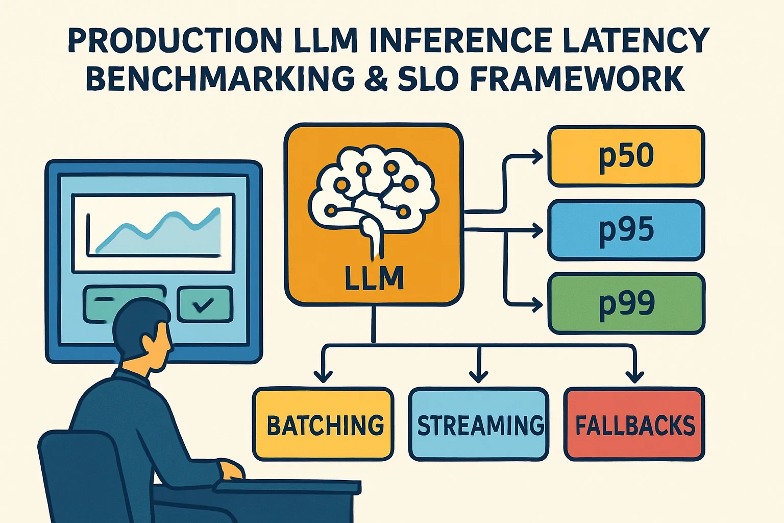
Dashboard chart showing p50, p95, p99 latency for batching, streaming, and fallback routes

Production teams don’t fail because the model is “slow”—they fail because latency is unpredictable and the system has no measurable contract (SLO/SLI) for p50/p95/p99, batching vs streaming behavior, and safe fallbacks.

In this article, you’ll get an evidence-led, production-grade approach to LLM inference latency benchmarking and an LLM inference SLO framework that explicitly covers streaming, batching, and fallback paths—so you can set SLIs that match user experience and catch regressions before customers feel them. If your LLM pipeline includes retrieval, you’ll also want to ensure RAG evaluation in production metrics doesn’t add hidden tail latency.

Failure scenario (what this prevents): A chatbot releases a “faster” model. In reality, end-to-end p99 latency balloons during peak traffic because token generation stalls under queueing and GPU contention. Worse, your metrics track only “time-to-first-token,” so you miss the long tail: users wait minutes for the full answer, timeouts spike, and the system silently retries downstream calls (amplifying load). Without a benchmark harness and a p99 SLO tied to end-to-end user latency, you ship the regression and only discover it through support tickets.

Executive Summary

TL;DR: Benchmark end-to-end LLM inference latency with explicit p50/p95/p99 SLIs, then enforce an LLM inference SLO framework that accounts for batching, streaming, and fallbacks—not just raw model speed.

Define SLI(s) that map to UX: usually time-to-first-token (TTFT) and time-to-last-token (TTLT), plus overall request latency for non-streaming clients.
Use benchmarking that separates compute latency (token generation) from system latency (queueing, retries, network, scheduling).
Model tail behavior: p99 is dominated by queueing + contention + worst-case decoding steps, so measure it under realistic concurrency.
Choose batching vs streaming based on a quantifiable trade-off: batching improves throughput but can worsen p95/p99 latency; streaming reduces perceived latency but can hide long TTFT→TTLT gaps.
Implement fallbacks with latency-aware routing (e.g., degraded model, smaller max tokens, tighter sampling) and test their impact on p99 latency SLOs.

Likely direct Q→A pairs

Q: What should my latency SLI be for streaming chat? A: Track both TTFT and TTLT (and/or full request latency) and alert on p95/p99 for each.
Q: How do batching and streaming change LLM latency? A: Batching boosts throughput but increases queueing (worse tails); streaming reduces perceived wait via early tokens but doesn’t eliminate p99 overall latency.
Q: What’s the minimum benchmarking setup for LLM inference latency benchmarking? A: Real model endpoints, realistic concurrency, token counts, and measurement of TTFT/TTLT plus end-to-end request latency.

How Production LLM Inference Benchmarking & SLO Framework Works Under the Hood

Think in layers: token decoding time (model compute) is only one part of latency. The rest is the serving system: batching policy, scheduling, queueing, networking, and client behavior (streaming consumption vs “wait for full response”).

1) Latency decomposition: compute vs system

For each request, capture timestamps:

t0: request received by your gateway/load balancer
t1: request enqueued/accepted by the inference server scheduler
t2: first token produced (TTFT event)
t3: last token produced (T T L T event)
t4: response fully delivered to client (end-to-end)

Then derive:

Queueing delay ≈ (t2 - t1) minus first-token compute portion; in practice you estimate by correlating load metrics (GPU utilization, batch queue depth) with TTFT.
TTFT = t2 - t0 (or t2 - t1 depending on measurement point).
TTLT = t3 - t0.
End-to-end request latency = t4 - t0.

Editorial discipline: If you only measure TTFT, you can ship a system that “starts fast” but finishes extremely late (p99 T T L T regresses). If you only measure end-to-end, you can’t reason about whether the tail is from queueing or from decoding length/sampling behavior.

2) Streaming vs batch: two different UX and two different measurement contracts

Streaming changes what “latency” means:

Perceived latency correlates strongly with TTFT.
Completion latency correlates with TTLT and end-to-end.

Batching changes what “latency” means operationally:

Requests may wait in a batch queue to be combined into a GPU-efficient batch.
Throughput improves; tail latency often worsens due to queueing under load, especially when max tokens vary across requests.

That’s why your SLO framework must specify which measurement regime it targets: streaming SLI (TTFT/TTLT) and non-streaming SLI (end-to-end).

3) p50/p95/p99 SLO design: what you promise and to whom

An LLM inference SLO framework works when the SLI is:

Observable in production
Actionable (you can change something to improve it)
Stable enough to avoid flapping due to measurement noise

Typical SLO structure:

Objective: e.g., “99% of requests complete within X ms over 28 days.”
SLI definition: e.g., end-to-end latency for non-streaming; for streaming, p99(TTLT) and optionally p99(TTFT).
Burn-rate alerting: page when error budget burn exceeds thresholds.

Important: For LLMs, “error” isn’t only HTTP 5xx. It includes latency violations, timeout fallback activations, and truncation if your product treats incomplete outputs as failures.

4) Benchmark harness: make latency falsifiable

To do credible LLM inference latency benchmarking, you need measurement that can distinguish:

Latency distribution changes due to your model/params (max tokens, temperature, top-p)
Latency distribution changes due to system factors (batch size policy, concurrency, GPU contention)
Measurement artifacts (wrong timestamping, buffering in the proxy, client not consuming stream)

A robust harness drives controlled scenarios and compares distributions statistically (not just averages). For tail metrics, use at least:

p50/p95/p99 for TTFT, TTLT, and end-to-end
concurrency sweeps (e.g., N=10, 50, 100, 200)
token length sweeps (short, medium, long outputs)
separate “warm” vs “cold” runs (cache effects, model load)

For teams building evaluation + ops for production LLMs, it’s worth pairing latency benchmarking with a broader evaluation discipline like our production RAG evaluation framework so you don’t optimize latency for the wrong user journeys.

Implementation: Production Patterns

Step 1: Instrument the right timestamps (don’t guess)

Implement timestamp logging at two points: ingress (gateway) and inference server. For streaming, instrument the “first token” and “last token” events at the server, then propagate them through your proxy.

Minimal metric set (per request):

model_id, route (stream/non-stream), prompt_tokens, output_tokens_target, output_tokens_actual
ttft_ms, ttl t_ms, end_to_end_ms
queue_wait_ms (or an estimate), retry_count, fallback_used (boolean)
http_status, client_abort (boolean)

Step 2: Define SLI(s) explicitly by route

A practical SLI mapping:

Streaming endpoint:
- SLI A: p99(TTFT) ≤ SLO_TTFT_MS (for perceived responsiveness)
- SLI B: p99(TTLT) ≤ SLO_TTLT_MS (for completion)
Non-streaming endpoint:
- SLI C: p99(end-to-end) ≤ SLO_E2E_MS

Recommendation: Always enforce at least one “completion” SLI (TTLT or end-to-end). TTFT-only SLOs are a common failure mode.

Step 3: Benchmark with realistic concurrency and token distributions

Drive a load profile that approximates production behavior. For example:

Users per minute with diurnal curve
Prompt size distribution (input tokens)
Output length distribution (requested max tokens and observed actual output)
Think time between turns for chat (impacts concurrency)

In benchmarks, you must also control or record sampling params (temperature, top-p) and decoding constraints (max tokens, stop sequences). These affect generation length and compute.

Step 4: Compare batching vs streaming latency under the same workload

For an apples-to-apples comparison, run identical load scenarios while varying:

server batching policy (max batch size, max waiting time, scheduling policy)
streaming on/off behavior (including proxy buffering)
client consumption behavior (ensure the client reads from the stream; don’t measure “server writes to a broken pipe”)

You’re looking for two curves:

Throughput vs p95/p99 latency
Concurrency saturation point where queueing dominates (p99 knee)

Step 5: Add latency-aware fallbacks and measure their SLO impact

Fallbacks should be triggered by latency budget signals, not just errors. Typical fallback actions:

Switch to a smaller model (or lower-cost endpoint)
Reduce max_tokens for the completion leg
Fallback to a deterministic decoding profile to reduce variance
Return partial output if your product supports it

Production contract: Fallback usage must be observable and reflected in SLI (e.g., count as failure if output is unacceptable).

Code: log TTFT/TTLT in a streaming server (pattern)

// Pseudocode: server-side instrumentation for streaming token events
// Goal: capture TTFT (time to first token) and TTLT (time to last token)

timestamp t0 = now();
startTrace(requestId);

boolean firstTokenEmitted = false;
timestamp ttft;

int tokensSent = 0;
for (token in model.streamGenerate(prompt, params)) {
  if (!firstTokenEmitted) {
    ttft = now();
    firstTokenEmitted = true;
    emitMetric("ttft_ms", (ttft - t0));
  }

  writeToStream(token);
  tokensSent++;
}

timestamp tEnd = now();
emitMetric("ttlt_ms", (tEnd - t0));
emitMetric("output_tokens_actual", tokensSent);
emitMetric("end_to_end_ms", (tEnd - requestIngressTime));

Code: define SLO evaluation queries (pseudo-PromQL)

// Pseudocode. Adapt to your metrics backend.
// Key idea: compute p99 for ttft_ms and ttl t_ms per route/model.

p99_over_time(ttft_ms{route="stream",model="gpt-x"}[5m])

p99_over_time(ttlt_ms{route="stream",model="gpt-x"}[5m])

p99_over_time(end_to_end_ms{route="non_stream",model="gpt-x"}[5m])

// SLO violation rule example:
// alert if p99(ttlt_ms) exceeds threshold
ALERT if p99(ttlt_ms) > SLO_TTLT_MS for 3 consecutive evaluation windows

Note: Not all time-series systems have native p99-over-time. If yours doesn’t, use histogram metrics (e.g., Prometheus buckets) to approximate p99 reliably, and validate approximation error in a staging environment.

Step 6: Close the loop with burn-rate alerts and runbooks

Use burn-rate alerts because LLM incidents are often short spikes. A typical runbook should include:

Verify whether the tail is queueing-driven or compute-driven (compare TTFT vs TTLT)
Check batching policy changes and GPU saturation metrics
Check retries and fallback activation rates
Confirm client aborts (don’t chase “latency” that is actually client disconnects)

If you’re also running RAG, you’ll want to ensure retrieval isn’t quietly adding latency spikes—pair your latency SLO work with RAG evaluation in production metrics & pitfalls so the tail doesn’t move unnoticed from generation to retrieval.

Comparisons & Decision Framework

Decision matrix: choose your latency SLOs based on UX contract

Use this quick comparison to decide what to measure and where:

If users care about first response quickly (chat feels responsive): enforce p99 TTFT alongside completion.
If users must receive complete answers within a time bound: enforce p99 TTLT (streaming) or p99 end-to-end (non-streaming).
If you do long-form generation: completion dominates; focus on TTLT/end-to-end and monitor distribution by output length bins.

Batching vs streaming latency comparison: a practical checklist

When comparing LLM batching vs streaming latency, don’t just look at averages—look at the knee point and tail drivers.

Hold constant: model weights, quantization, tokenizer, decoding params, output token cap.
Run concurrency sweeps: identify where p99 rises sharply (queueing saturation).
Compare TTFT: streaming should reduce TTFT under normal load; if it doesn’t, suspect proxy buffering or scheduling.
Compare TTLT: batching may degrade TTLT due to waiting; streaming may not fix it if completion compute is still delayed.
Quantify user-impact: if you have a UI that renders tokens as they arrive, TTFT matters; if the UI waits for completion, end-to-end dominates.

Example target SLO shape (template)

Choose thresholds based on your product and typical usage lengths. A template:

Streaming chat: p99 TTFT ≤ 1200ms, p99 TTLT ≤ 8000ms
Non-streaming: p99 end-to-end ≤ 9000ms

Then set burn-rate alert thresholds and error budget windows (e.g., 28-day objective with short/long burn alerts).

Failure Modes & Edge Cases

1) p99 hiding behind “average speed improvements”

Failure pattern: a new model reduces mean decode time, but the tail gets worse due to increased output length variance or scheduling interactions.

Diagnostic: break down p99 by output token bins (e.g., <64, 64–256, >256 tokens). If the knee is bin-dependent, your SLO must encode that reality (or enforce output caps).

2) TTFT-only SLOs that greenlight broken completions

Failure pattern: server streams first token quickly, but later tokens stall (e.g., GPU fragmentation, cache misses, contention in post-processing).

Diagnostic: compare TTFT vs TTLT percentiles. If TTFT is stable but TTLT p99 degrades, focus on decode throughput and completion path.

3) Proxy buffering & client consumption artifacts

Failure pattern: streaming is “enabled,” but intermediate proxies buffer chunks, so the client receives the first token late.

Diagnostic: measure TTFT at server and at client. If client TTFT >> server TTFT, your network/proxy layer is the culprit.

4) Batching policy regressions at peak load

Failure pattern: batching max-wait increases, or batch formation gets less efficient as request lengths diverge.

Diagnostic: correlate p99 spikes with batch queue depth and batch formation efficiency (tokens per batch, padding ratio). Tune scheduling: reduce max-wait or add length-aware grouping.

5) Fallback loops and amplified load

Failure pattern: timeouts trigger fallbacks, which trigger retries, which increase load, worsening latency—classic positive feedback loop.

Diagnostic: track retry_count and fallback_used alongside latency. Add circuit breakers: once fallback is used, don’t retry the same failing path.

For more production reliability considerations that intersect with risk, see our threat modeling approach for LLM security testing—many “latency incidents” are actually induced by abuse patterns (e.g., prompt flooding, resource exhaustion).

6) Measurement noise and histogram drift

Failure pattern: p99 estimates fluctuate due to sparse traffic or incorrect histogram bucket configuration.

Mitigation: run benchmarks long enough, validate p99 error bounds in staging, and ensure consistent timestamping (monotonic clocks).

Performance & Scaling

What p50/p95/p99 typically tell you

p50: baseline performance—good for tracking model changes and straightforward compute regressions.
p95: user-visible issues during moderate load; often influenced by queueing growth.
p99: tail sensitivity—dominated by queueing saturation, worst-case output lengths, and rare contention events.

Benchmark guidance: how many samples and how to bin

To make p99 meaningful:

Ensure enough requests per latency bin to stabilize the tail (especially in CI).
Bin by output token length (requested and actual) and route (stream vs non-stream).
Capture at least 2–3 concurrency points around the expected saturation knee.

Key KPIs to monitor alongside latency

GPU utilization and memory headroom (OOM risk can cause sudden tail spikes)
KV cache hit rate (if supported by your server)
Batch queue depth and max wait time settings
Tokens/sec and effective tokens/sec per batch
Timeouts, retries, fallback rate
Client abort rate

Scaling lever map (from symptom to lever)

p99 TTFT high → reduce queueing: lower batch max-wait, increase replicas, improve scheduling, inspect ingress throttles.
p99 TTLT high → improve decode throughput: tune max tokens, reduce post-processing overhead, check quantization and decoding settings.
p99 end-to-end high only for non-streaming → streaming could improve perceived latency; check proxy buffering and response assembly.
Latency spikes correlate with retries/fallbacks → add circuit breakers; cap retries; ensure fallback output isn’t itself causing rejections.

Production Best Practices

1) Rollouts: gate on p95/p99, not mean

Use canary releases and gate promotions on tail metrics for your primary route(s). A disciplined rollout checks:

p99 TTFT and p99 TTLT (streaming) remain within budget
fallback rates don’t increase materially
error budgets aren’t consumed too rapidly

2) Test your fallbacks like you test the main path

Fallbacks are not “just for emergencies”—they are part of the SLO contract. Bench them explicitly:

Fallback model latency distribution
Effect on output length (often shorter) and user acceptance
Whether fallback reduces or increases system load

3) Keep latency measurement consistent across staging and prod

Common pitfall: staging has different proxy behavior or different batch settings. Ensure your staging benchmark harness uses the same:

routing stack
proxy buffering configuration
batching policy parameters
token limits and decoding params

4) Pair latency SLOs with retrieval and safety testing when applicable

Latency in LLM systems often includes RAG retrieval. To avoid chasing phantom tail regressions, align latency SLO instrumentation with your evaluation metrics; start with the RAG evaluation checklist for production systems to ensure you’re measuring what users actually experience.

Appendix: A Benchmark Scenario Template (Copy/Paste)

If you want a repeatable harness, define scenarios with explicit parameters:

Route: streaming, non-streaming
Concurrency: 25, 50, 100, 200 concurrent inflight requests
Prompt tokens: short/medium/long prompts
Output tokens: max_tokens = 64/256/1024; measure actual output
Decoding: temperature, top_p, stop sequences
Batching policy: max_wait_ms, max_batch_size, scheduler mode
Fallback: off (baseline) and on (latency-aware)

Then generate reports: p50/p95/p99 for TTFT, TTLT, and end-to-end; plus a “tail driver” section that attributes p99 spikes to queueing vs decode length by correlation.