Edge Computing IoT Battery Life: Practical Strategies

26 Mar, 2026

Introduction

IoT sensors connected to edge gateway, battery icon, cloud link diagram on screen.

Problem statement: In production IoT deployments, battery life drives maintenance cost, user experience, and feasibility; extending device runtime while preserving functionality requires system-level design, not just smaller components.

What this article delivers: A practical, production-tested set of edge computing strategies — from duty-cycle and sleep scheduling through TinyML inference placement and radio optimization — that engineers can implement and measure to extend device battery life.

Failure scenario: A fleet of battery-powered environmental sensors deployed in a remote agricultural site begins showing a 30-50% reduction in expected runtime after a firmware update. Devices run periodic sampling and either send raw data every minute or run a local classifier. Troubleshooting reveals the update increased wake time (longer sensor stabilization), increased flash wear from frequent logging, and enabled a high-frequency heartbeat to the cloud. Without a rollback the fleet requires costly truck-rolls to replace batteries. This article prevents and mitigates such outcomes by prescribing design patterns, diagnostics and safe rollout practices.

Executive Summary

TL;DR: Shift computation to the edge selectively, optimize sensing and radio duty cycles, and use TinyML and adaptive sampling to reduce energy per useful decision by 2x–10x depending on workload.

Place simple inference at the device when it prevents radio transmissions; reserve cloud only for heavy retraining or coordination.
Energy cost is dominated by radio activity and memory access — not compute — for many IoT platforms; optimize both.
Combine hardware low-power modes, interrupt-driven wakeups, and coalesced transmissions (batching) to reduce idle current and radio on-time.
TinyML quantization + pruning reduces inference energy; run models at lower fidelity adaptively when conditions allow.
Use realistic energy models (E = V * I * t) and p95/p99 SLAs to plan battery replacement cycles and design runbooks.

Three likely quick Q→A pairs

Q: Where should I run inference to save the most energy? A: Run lightweight inference on-device when it avoids at least one radio transmission per decision.
Q: Is the radio or CPU more expensive? A: For typical narrowband radios, radio Tx dominates energy per bit; CPU memory accesses can be comparable if models exceed cache and cause flash reads.
Q: What single change gives the biggest battery gain? A: Reduce radio duty cycle through batching/coalescing and event-driven wakeups; this often yields the most immediate ROI.

How Edge computing strategies to extend IoT device battery life Works Under the Hood

At system level, energy optimization is a multi-dimensional problem: sensing frequency, local compute (inference), memory access pattern, radio use, and peripheral power all interact. The common architecture is three-tiered:

Device (sensor + MCU + radio): runs fast, deterministic TinyML models, hardware timers, and a local power-management controller.
Edge gateway or fog node (optional): aggregates, provides connectivity, and can run heavier models or coordinate devices to reduce redundant transmissions.
Cloud: long-term storage, retraining, fleet analytics and OTA update delivery.

Key algorithms and protocols used in practice:

Interrupt-driven sleep scheduling: MCU sleeps in deep low-power mode and wakes on GPIO/timer/DMA events.
Event-triggered TinyML inference: sensor preprocessors generate compact feature vectors (e.g., MFCCs, power envelopes) that feed quantized models.
Adaptive sampling and fidelity switching: sample rate and model size change based on context (time of day, battery level, recent alarms).
Batching & coalescing: buffer events locally and send them in fewer radio sessions to amortize radio startup cost.
Energy-aware network protocols: use CoAP/DTLS or MQTT-SN with low-power optimizations (sleep-friendly keepalive, piggybacked ACKs).

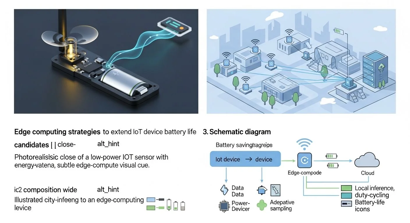
Diagram (text): Device sensors -> prefilter/feature extractor -> TinyML (quantized) -> decision: keep/local log OR wake radio to transmit summarized event -> Edge gateway aggregates -> Cloud. Hardware blocks (ADC, DMA, RTC, radio, flash) are power-managed at the driver level: ADC and DMA run briefly, DMA writes into RAM, MCU only wakes for inference or critical handling, radio powered on only for scheduled transmissions.

Implementation: Production Patterns

I present a progressive set of patterns: Basic, Advanced, Error handling, and Optimization. Where appropriate I include code snippets for Cortex-M + TF Lite Micro and for server-side duty-cycle estimation.

Basic pattern: Interrupt-driven sensing and coalesced upload

Keep the MCU in deepest sleep state between events (stop or standby modes on Cortex-M).
Use DMA + peripheral sampling so CPU doesn't spin on ADC reads.
On event, wake, sample N readings, run simple threshold or a TinyML model, then either store locally or open radio for a single, batched upload.

Rationale: The radio state transition (wake, sync, handshake, Tx) often costs more energy than a few inference cycles. Coalesce when possible.

Advanced pattern: Adaptive TinyML and fidelity switching

Deploy two-tier models: a tiny, always-on classifier (e.g., 8-bit quantized) and a larger model that runs only when the tiny model signals uncertainty.
Use confidence thresholds to trade CPU vs radio: if local classifier is confident and indicates "no action", skip transmission; otherwise send summary or wake gateway for heavier inferencing.
Adapt sample rate based on battery voltage, recent activity, and time-of-day schedules.

Place to link related material: For a deep dive on TinyML and Cortex-M deployment patterns, see practical strategies for TinyML and TF Lite Micro on constrained MCUs, which covers quantization and runtime memory trade-offs.

Code: Minimal low-power inference loop (C, Cortex-M, TF Lite Micro)

#include "tensorflow/lite/micro/all_ops_resolver.h"
#include "tensorflow/lite/micro/micro_interpreter.h"
#include "model_data.h" // compiled quantized model

// Pseudocode: platform-specific sleep/wake and radio API abstracted
void main() {
  platform_init_low_power();
  setup_adc_dma_sample_buffer();
  setup_rtc_wakeup();

  while (1) {
    platform_sleep_deep(); // wait for DMA complete or GPIO wake

    if (dma_buffer_ready()) {
      float features[FEATURE_DIM];
      extract_features_from_dma(features);

      uint8_t input_quantized[INPUT_BYTES];
      quantize_features(features, input_quantized);

      // TF Lite Micro inference (preallocated arena)
      TfLiteStatus invoke_status = run_tflm_inference(input_quantized);

      if (is_event_detected()) {
        // either buffer locally or open radio for a coalesced upload
        buffer_event_locally_or_schedule_tx();
      }
    }

    // optional periodic telemetry
    if (periodic_timer_elapsed()) {
      open_radio_and_send_telemetry();
    }
  }
}

Notes: keep the interpreter arena in RAM and avoid dynamic allocations; ensure model fits in RAM or use execute-in-place strategies to avoid flash page activations during inference.

Server-side pattern: battery life projection and coalescing scheduler (Python)

# Estimate energy per event and plan batch windows
V = 3.3  # nominal voltage
I_radio_tx = 0.050  # A during Tx (50 mA)
I_radio_rx = 0.030  # A during Rx
I_mcu_sleep = 0.00002 # A (20 uA in deep sleep)
I_mcu_active = 0.005  # A (5 mA during active processing)

# durations (s)
T_radio_startup = 0.2
T_tx_per_byte = 0.002
payload_size = 20

E_radio = V * (I_radio_tx * (T_radio_startup + payload_size * T_tx_per_byte))
E_mcu_infer = V * I_mcu_active * 0.05  # 50 ms inference
E_sleep_per_day = V * I_mcu_sleep * 86400

print('radio energy per upload (J):', E_radio)
print('inference energy (J):', E_mcu_infer)
print('sleep energy/day (J):', E_sleep_per_day)

# Use these to compute mAh/day and projected battery lifetime

Use server-side telemetry to compute p95/p99 energy per device and tune batch windows appropriately; implement remote configuration for batch window size and sample rate.

Error handling and safe fallbacks

Always include a minimal mode that disables non-essential sensing and reduces uplink frequency when battery falls below a safe threshold.
On inference failure (out-of-memory, model panic), revert to a conservative threshold-based detector rather than enabling continuous radio or CPU spinning.
Deploy OTA with staged rollouts and canary groups; allow rollback if fleet-wide battery regression is observed.

Comparisons & Decision Framework

Edge vs cloud trade-offs are about energy, latency, and model complexity. Below is a decision checklist and a compact trade-off table.

Decision checklist

Do you avoid at least one radio transmission for each on-device inference? If yes, local inference usually saves energy.
Can the model fit in RAM without frequent flash access? If not, consider model compression or execute-in-place techniques.
Is latency critical (sub-second)? If yes, edge inference reduces round-trip time and often energy by avoiding retransmissions.
Do devices operate in intermittent connectivity? Edge-first designs with opportunistic sync are preferable.
Is fleet-wide model drift expected? Use hybrid approaches where cloud triggers model refresh and a smaller local model handles day-to-day operations.

Trade-offs summary

Local TinyML: +Low radio usage, +Low latency, -Constrained model size/accuracy, +Resilient offline
Gateway inference: +Aggregate redundancy removal, +Better compute, -Adds hop and complexity, +/- energy depends on link
Cloud inference: +High accuracy and easy updates, -High radio energy and latency, -Requires connectivity

Failure Modes & Edge Cases

Common failure modes with diagnostics and mitigations:

High idle current: symptom: battery drains linearly even when device idle. Diagnose with on-device current logging or bench power meter measuring sleep current. Mitigation: ensure MCU enters deepest sleep, disable peripherals, fix errant timers, and check for debug UART left enabled.
Flash thrashing / long boot: symptom: long current spikes on wake. Diagnose: inspect boot sequence, check file-system wear or logging frequency. Mitigation: move frequently-written logs to FRAM or circular buffer in RAM, defer defragmentation operations to maintenance windows.
Radio retransmit storms: symptom: many small packets instead of batched uploads. Diagnose: network logs, count ACKs and retries. Mitigation: implement exponential backoff, larger MTUs, and application-layer deduplication; prefer robust link-layer like 802.15.4 with ACKs.
Model execution causing memory faults: symptom: device reboots after model infer. Diagnose: capture crash logs, enable minimal logging to flash, reproduce in hardware debugger. Mitigation: validate model size vs RAM, enable stack and heap usage checks, preflight memory allocation on startup.
Clock drift causing missed wake windows: symptom: scheduled transmissions fail or collide. Diagnose: compare RTC against gateway time, check temperature sensitivity. Mitigation: use high-accuracy RTC or periodic synchronization, apply jitter to avoid collisions.

Performance & Scaling

Benchmarks to measure and SLAs to set. Design KPIs, p95/p99 guidance and monitoring suggestions.

Core KPIs

Average current draw (uA/mA) in sleep, active, and radio Tx/Rx states.
Energy per useful decision (J/decision).
mAh consumed per day (average) and projected battery lifetime (days) with p95/p99 bounds.
P95 inference latency and p99 end-to-end decision latency (including sensing, inference, and radio if applicable).
Packet success rate and retry count distribution.

Example target numbers (production-calibrated ranges)

Sleep current: <50 uA for long-lifetime sensors (coin cell/AA months).
Active inference duration: 10–200 ms depending on model size and MCU speed.
Radio session startup + Tx: 100–500 ms (LoRaWAN tends to have longer link time; BLE is shorter but depends on connection parameters).
Energy per upload (20–200 bytes): 10–200 mJ depending on radio.
Battery life improvement target from edge strategies: 2x–10x vs naive periodic uplink every sample.

Set p95/p99 SLAs on energy per decision: track distribution across fleet and alert when p95 exceeds expected envelope by a configurable multiplier (e.g., 1.5x baseline) which indicates a regression or environmental change.

Monitoring recommendations

Telemetry: periodic battery voltage, uptime counters, event counts, and radio retries. Use compression or sparse telemetry if cost sensitive.
Edge gateway metrics: aggregated per-device batch size distribution and peak upload times to detect coalescing failures.
Use synthetic canaries: devices that exercise full-stack behavior with known inputs to detect drift in inference energy or latency.

Production Best Practices

Security, testing, rollout and runbook items that reduce risk when optimizing for battery life.

Security: minimize always-on connectivity and avoid long-lived credentials; use ephemeral session keys or DTLS with sleep-friendly rekey intervals. Ensure OTA updates are signed and verify on device to avoid power-wasting malicious payloads.
Testing: create lab power profiles and run soak tests across temperature ranges; validate inference accuracy after quantization and under representative noise.
Rollout: staged OTA with small canary group, monitor p95 battery consumption and rollback on negative trend. Use feature flags to reduce exposure.
Runbooks: define clear procedures for when battery regression occurs: identify canary group, collect minidumps, roll back firmware, temporarily enable minimal mode, and schedule physical intervention if necessary.
Documentation: record per-device energy models (sleep current, active currents, radio cost) and include them in procurement and acceptance tests.

Appendix: Quick energy math and a checklist

Energy calculations you can reuse. Electrical basics:

Energy (Joules) = Voltage (V) * Current (A) * Time (s)
1 mAh at 3.3 V ≈ 3.3 * 3.6 = 11.88 Joules (since 1 mAh = 1/1000 A for 3600 seconds)

Example projection: A device with 200 uA sleep, two 50 ms inferences per day at 5 mA, and one 200 ms radio Tx at 50 mA per day:

Sleep energy/day: 3.3 V * 0.0002 A * 86400 s = 57.0 J (~4.8 mAh)
Inference energy: 3.3 * 0.005 * 0.1 s = 0.00165 J (~0.00014 mAh) negligible compared to radio
Radio energy: 3.3 * 0.05 * 0.2 = 0.033 J (~0.0028 mAh) — but if startup time is larger or multiple transmissions occur, radio dominates

Checklist before deployment:

Measure idle (sleep) current on hardware revision.
Estimate and measure radio startup overhead and per-byte Tx cost.
Validate model memory footprint and measure inference time & energy in lab.
Implement battery-safe fallback and minimal mode.
Plan OTA staged rollout and telemetry to detect battery regressions quickly.

Closing: Practical next steps

Start with the telemetry you need to measure energy — battery voltage, sleep/active counters and radio retries. Implement a minimal on-device classifier that blocks one periodic uplink and quantify the actual battery savings in a small pilot. Use the energy math above to model fleet-level replacement cycles and apply staged OTA rollouts. For hands-on TinyML and Cortex-M guidance during implementation, review the practical TinyML and TF Lite Micro strategies which include memory and runtime optimizations that directly impact power consumption.

MAKB editorial note: In the field, the most common failure we see is optimistic assumptions about sleep current and radio costs. Measure before you optimize, instrument during rollout, and make the conservative path (minimal mode) trivial to enable remotely.

Edge Computing IoT Battery Life: Practical Strategies

Introduction