Edge computing IoT battery life optimization — Practical Guide

Introduction

Problem statement: In production IoT fleets, battery replacement or recharging drives the cost of ownership and often limits deployment feasibility.

What this article delivers: A pragmatic, engineer-focused playbook for using edge computing and TinyML techniques to measurably extend IoT device battery life, with patterns, code, diagnostics, and p95/p99 guidance for production.

Failure scenario (example): A distributed sensor fleet deployed in logistics reports intermittent 30% battery-life degradation versus lab estimates. Initial root-cause assumptions point to Radio duty cycle, but analysis shows excessive wake-ups caused by local pre-processing and non-optimized inference—leading to both CPU and radio energy waste. Without a coordinated edge strategy (low-power inference, adaptive sleep scheduling, and well-placed offload points), devices fail to meet p95 operational lifetime targets and trigger costly field maintenance.

Executive Summary

TL;DR: Offload work intelligently and run only the smallest, most accurate models locally; pair low-power edge inference with event-driven sleep schedules and lightweight coordination layers to push device energy consumption to its fundamental limits.

• Run tiny models at the edge (quantized TinyML) only when necessary; prefer feature extraction in hardware where possible.
• Use adaptive, event-driven sleep scheduling with radio coalescing to reduce wake-up frequency (target <1% active duty-cycle for many sensors).
• Make offload decisions with a cost model: compare local compute energy vs. transmit energy + latency SLA.
• Profile at p95/p99 (not mean): design for worst realistic duty cycles. Measure CPU, radio Tx/Rx, and sensor acquisition costs separately.
• Implement incremental rollouts, runtime telemetry, and power-aware firmware updates to avoid regressions in the field.

Three likely direct Q→A pairs

• Q: How much energy can you save with edge inference vs. always sending raw data? A: Typical savings are 5x–50x depending on model size and radio cost; quantized 8-bit models on Cortex-M can cost microjoules per inference vs. millijoules to transmit.
• Q: When should you offload to a gateway rather than run locally? A: Offload when transmit energy + latency allowance < local compute energy for the class of workloads or when model size exceeds device constraints; use a runtime energy cost estimation to decide.
• Q: What's the highest-impact single change to improve battery life? A: Reduce radio transmissions via edge filtering and batching; radios dominate energy in most low-duty sensors.

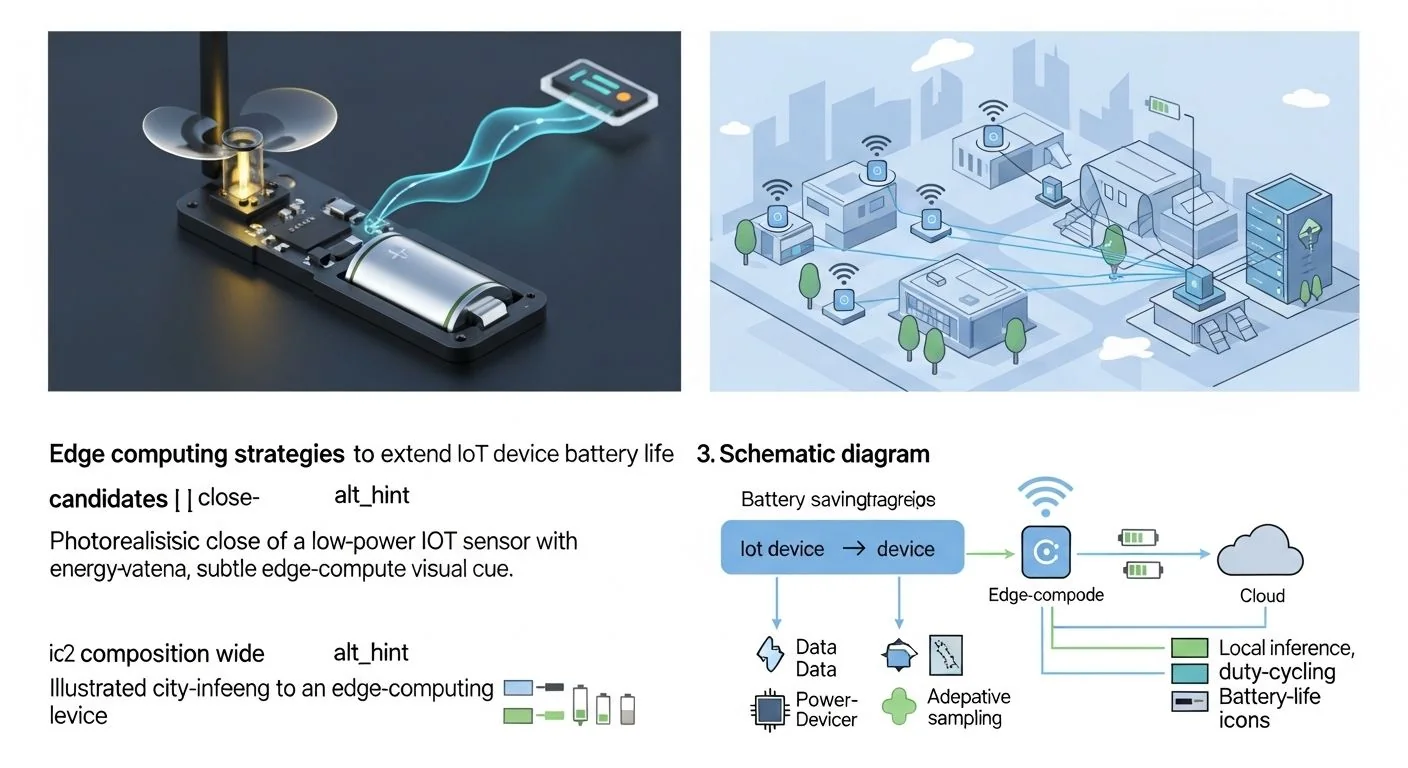
How Edge computing strategies to extend IoT device battery life Works Under the Hood

Architecture summary: The pattern splits responsibility across three layers—device, local edge/gateway, and cloud. Devices run ultra-low-power routines: sensor acquisition, minimal feature extraction, and a tiny classifier or trigger. Gateways aggregate, run higher-compute models, and manage coordination. The cloud handles long-term model training, fleet analytics, and policy distribution.

Key algorithms/protocols:

• Low-power inference: Quantized neural networks (8-bit, integer-only inference), optimized kernels for Cortex-M (CMSIS-NN, TF Lite Micro), and KD-tree or lightweight classical algorithms where applicable.
• Sleep scheduling: Event-driven deep sleep with hardware timers and interrupt-on-change. Use grouped wake windows (radio coalescing) and randomized jitter to prevent synchronized storms.
• Offload decision model: Cost(E_compute_local, E_tx, latency) = choose local if E_compute_local + penalty(local_miss) < E_tx + penalty(offload_latency).
• Radio optimization: Use compressed payloads, adaptive retransmit windows, and link-layer duty-cycling (e.g., IEEE 802.15.4 MAC layer tweaks or Bluetooth LE connection parameter tuning).

Diagram as text: Device [Sensors + MCU + Radio] -> Gateway [Edge server with GPU/CPU] -> Cloud. Device runs Sensor Acquisition -> Feature Extractor -> TinyML Trigger -> (if event) Radio Tx -> Gateway processes and may request full payload or send policy updates back to device.

Implementation: Production Patterns

We structure implementation as basic → advanced → error handling → optimization. The examples assume an Arm Cortex-M class device, TF Lite Micro, and a lightweight MQTT/CoAP gateway.

Basic pattern — sensor filter + trigger

1. Measure and document baseline power profile (idle, active sampling, inference, Tx). Use a high-resolution power monitor (e.g., Monsoon Power Monitor or Nordic Power Profiler Kit).
2. Implement hardware-driven sampling and interrupts: configure ADC/DMA or peripheral to sample without CPU where possible.
3. Run simple threshold or lightweight model (e.g., decision tree) in RAM to filter events before radio use.

// Pseudocode: interrupt-driven threshold filter (C-like)
void sensor_isr(void) {
    uint16_t sample = adc_read();
    if (sample > EVENT_THRESHOLD) {
        record_event(sample);
        schedule_inference(); // wake main loop briefly
    }
}

Advanced pattern — TinyML + offload decision

Use a tiny quantized model (<=50 KB) for on-device inference. Combine with a runtime energy estimator to decide whether to send full samples or just the event.

// Pseudocode: energy-based offload decision
float estimate_local_compute_joules(int model_ops) { return model_ops * ops_to_joules; }
float estimate_tx_joules(int bytes) { return bytes * bytes_to_joules + radio_wakeup_joules; }

void handle_event(samples_t *s) {
    int ops = model_ops_for_inference();
    float localE = estimate_local_compute_joules(ops);
    float txE = estimate_tx_joules(min_payload_bytes);
    if (localE < txE) {
        int8_t result = tinyml_infer(s); // run local model
        if (result == POSITIVE) send_event_summary(result);
    } else {
        send_raw_or_compressed(s);
    }
}

Notes: Calibrate ops_to_joules and bytes_to_joules per device using empirical profiling. Update these constants with firmware OTA when hardware changes.

Error handling and resilience

• Graceful fallbacks: If model execution fails (stack overflow, memory fault) revert to a safe threshold-based filter to avoid spurious radio usage.
• Watchdog and power-safe state: Ensure watchdog resets preserve minimal duty cycle behavior and avoid prolonged CPU spin loops consuming energy.
• OTA robustness: Use delta updates and atomic swap to avoid bricking devices when shipping new inference kernels or quantized models.

Optimization steps (practical sequence)

1. Profile and quantify breakdown: sensor acquisition, preprocessing, inference, radio Tx/Rx, idle sleep current. Aim for a clear cost table (microjoules per operation).
2. Reduce radio wake-ups: apply edge filtering and batching to reduce transmissions by 90%+ where acceptable.
3. Shrink model: prune, quantize, and use depthwise separable layers. Benchmarks: pruning to 50% weights often reduces ops ~2x with minor accuracy loss.
4. Use hardware accelerators: CMSIS-NN or vendor DSP intrinsics reduce inference energy by 2x–5x vs. naive C implementations.
5. Software tweaks: eliminate dynamic memory, align buffers, place frequently-used code/data in tightly-coupled memory to reduce cycles and power.

Comparisons & Decision Framework

Choice axes: local-only vs. hybrid (edge/gateway) vs. cloud-only. Use this checklist to decide:

• Energy cost of Tx vs. compute on device (measure!). If Tx >> compute, prefer local processing.
• Latency SLA: Critical real-time decision often requires local inference.
• Model update cadence: If models need frequent updates, consider hybrid to reduce OTA churn.
• Security/Privacy: Sensitive data may require on-device processing.
• Hardware constraints: memory, compute, and accelerators determine feasible model families.

Trade-offs table (summary)

• Local-only: Lowest network cost, minimal latency, highest OTA complexity, model size constrained.
• Hybrid (gateway): Best balance—device runs tiny triggers, gateway runs heavier models and manages aggregation; slightly higher network usage but better accuracy and easier retraining.
• Cloud-only: Highest energy cost from devices, best model flexibility, easiest model ops and monitoring, but often impractical for battery-constrained devices.

Failure Modes & Edge Cases

Below are concrete diagnostics and mitigations for the top failure modes seen in production fleets.

1. Unexpected battery drain

Diagnostics: Collect per-device telemetry—uptime, wake counts, tx counts, CPU active time. Compare p95 wake-up rate with expectation. Tools: instrumented firmware and periodic debug logs (compact, compressed).

Mitigation: If radio wake-ups are high, introduce batching or increase filter sensitivity. If CPU active time is high during inference, profile for memory thrashing or unexpected interrupts causing wake-ups.

2. Model drift causing excess false positives

Diagnostics: Compare local model outputs vs. gateway/classifier outputs on sampled payloads. Track false positive rate at p95.

Mitigation: Use gateway validation to collect labeled failure cases and push incremental retrains. Introduce adaptive thresholds that can be updated via lightweight parameter push.

3. OTA update causing higher power use

Diagnostics: After OTA, re-run power profile. Look for changes in sleep current (could indicate peripheral misconfigured) or increased timer interrupts.

Mitigation: Validate OTA in a staged rollout with telemetry rollback triggers. Keep a golden image and ensure delta update minimizes flash write energy and wear.

4. Synchronization storms

Diagnostics: Correlate battery drops across devices and timestamped gateway logs. If many devices wake simultaneously, likely scheduled maintenance or synchronized timers.

Mitigation: Add randomized jitter to wake windows. Use gateway-driven stagger policies for mass firmware restarts or policy pushes.

Performance & Scaling

KPIs to track (production):

• Device battery life median and p95 (target: p95 > target lifetime)
• Wake-ups per hour, radio transmissions per day
• Average inference energy (microjoules) and model runtime (ms)
• False positive/negative rates at device vs. gateway

Benchmarks & target guidance (practical numbers):

• Radio Tx of 50 bytes on BLE/LoRaWAN: ~1–50 mJ (device and radio dependent). For low-power radios, expect median ~5–20 mJ per Tx.
• Quantized 8-bit TF Lite Micro inference on Cortex-M4: ~10–100 μJ per inference for very small models (<= 50K params) using CMSIS-NN; naive implementations may be 5–10x worse.
• Idle deep sleep current: typical 1–10 μA for modern MCUs, but peripherals and sensor front-ends can increase this to 20–100 μA.
• Design rule: If a single Tx costs >100x an inference, prioritize local inference and reduce Tx frequency.

p95/p99 guidance: Design for p95 or p99 duty cycles, not average. For example, if typical wake-ups are 2/hour but p95 is 20/hour during spikes, ensure battery sizing and duty-cycle limits cover that spike profile without immediate failure.

Scaling considerations: Gateway capacity (both compute and network) must be planned: if each gateway handles N devices, estimate peak behavior (e.g., firmware rollouts or environmental triggers) and ensure autoscaling or rate-limiting of device check-ins. Prefer backpressure mechanisms and staggered rollout policies to avoid gateway overload.

Production Best Practices

• Security: Encrypt both model updates and payloads. Use secure boot and signed firmware to avoid malicious power-wasting firmware.
• Testing: Maintain a hardware-in-the-loop test bench with power monitors to validate energy claims before rollouts; run A/B experiments across device cohorts.
• Rollout: Staged canary releases with automated telemetry-based rollback. Release model parameter changes before binary changes when possible.
• Runbooks: Create a battery-runbook with steps to diagnose high drain (collect telemetry, check wake counts, check radio counts, check recent OTAs).
• Telemetry: Add compact power telemetry that reports counters (wake-ups, txs, inference count) weekly; avoid continuous high-bandwidth telemetry as it defeats the power-savings purpose.

Further Reading & References

• TensorFlow Lite Micro documentation — Practical guide to TinyML on microcontrollers, CMSIS-NN integration, and quantization techniques.
• TinyML Foundation resources — Community resources, benchmarks, and the TinyML book.
• ARM Cortex-M documentation — Microcontroller architectures and low-power features.
• Nordic Semiconductor: low-power wireless — Radio energy characteristics and power profiling tools.
• Selected IEEE papers on energy-efficient edge computing — For academic context on cost models and distributed inference trade-offs.

Additional internal resources: For concrete firmware patterns and TinyML tips used in production at our shop, see our guide to TinyML power efficiency best practices and for scheduling patterns consult our guide to IoT sleep scheduling algorithms which includes runnable scheduler templates and jitter strategies.

Appendix: Practical profiling checklist & minimal example

Profiling checklist (run before and after changes):

1. Measure sleep current (μA) with peripherals configured as in production.
2. Measure active sampling energy per sample (μJ/sample).
3. Measure inference energy per run and ms runtime; run with CMSIS-NN and without to compare.
4. Measure radio Tx energy for representative payloads (μJ/byte or mJ per message).
5. Estimate expected daily transmissions, inferences, and samples to compute daily energy and map to battery capacity.

// Minimal runtime energy estimator (pseudo-C)
#define BATTERY_CAPACITY_MJ (3.6f * 3600.0f) // e.g., 3.6V * 1Ah -> convert to mJ

float compute_daily_energy(int wakes_per_day, int inferences_per_wake, 
                           float inf_joules, float tx_joules_per_msg, int msgs_per_day,
                           float sleep_current_uA) {
    float activeE = wakes_per_day * inferences_per_wake * inf_joules + msgs_per_day * tx_joules_per_msg;
    float sleepE = sleep_current_uA * 1e-6f * 24.0f * 3600.0f; // J per day
    return (activeE + sleepE) * 1000.0f; // return mJ
}

// Use this to iterate scenarios and choose policies that keep energy < battery

Final note from the editor: prioritize empirical measurement. Theory and models guide decisions, but field telemetry (p95/p99) drives reliable battery-life optimization. Use the decision checklist, profile early, and adopt a staged rollout to protect device lifetime targets.