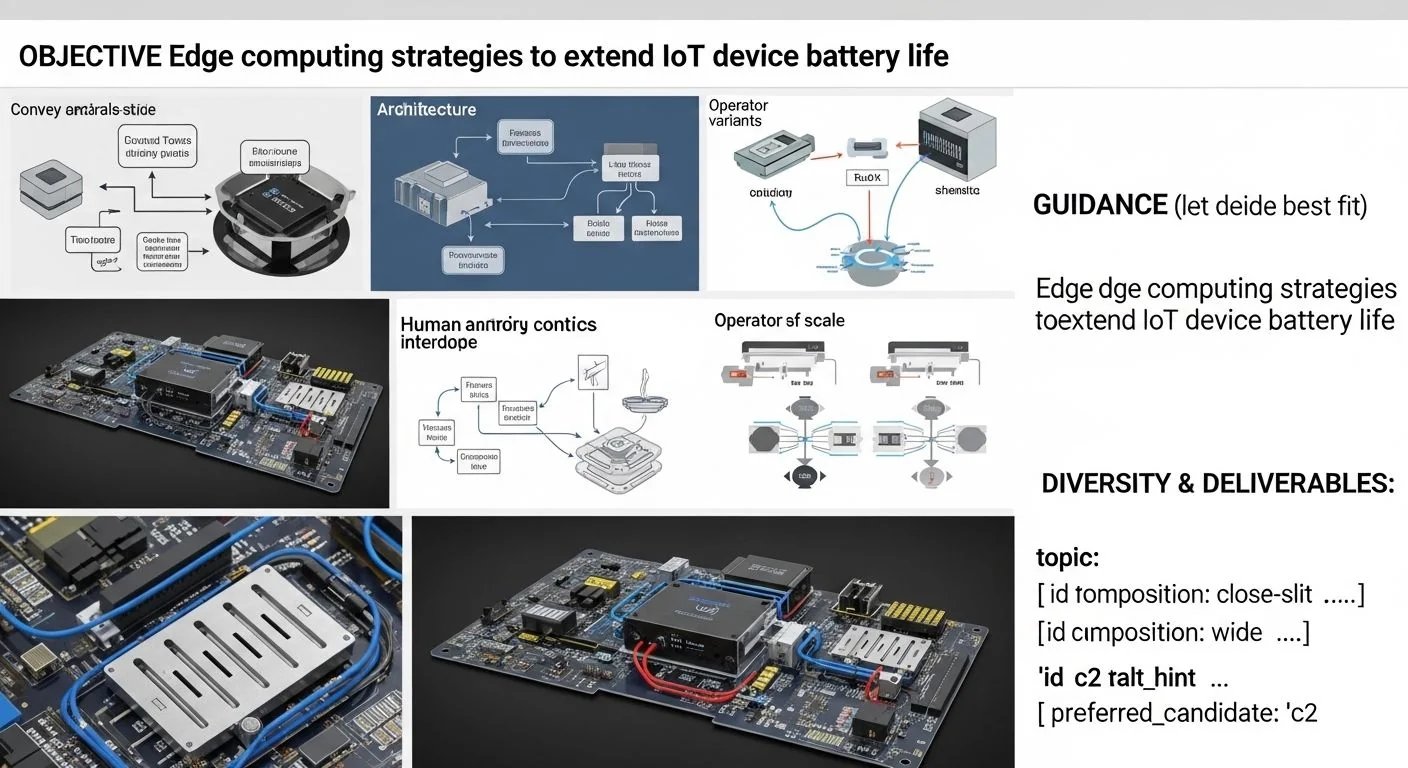
Edge Computing Strategies to Extend IoT Device Battery Life

19 Feb, 2026

Introduction

IoT sensors connected to edge gateway, battery icon, cloud link diagram on screen.

A typical industrial IoT sensor deployed in remote pipeline monitoring dies at 18 months instead of its designed 5-year lifespan—not from component failure, but from accelerated battery depletion caused by suboptimal communication patterns. The root cause: every sensor reading triggers an immediate cloud upload, burning 150-400 mJ per transmission over cellular LPWAN. When multiplied across 10,000+ devices, this architectural decision transforms a viable business case into a maintenance nightmare requiring truck rolls every two years.

This article delivers production-tested edge computing strategies that reduce per-event energy consumption by 60-95% through intelligent preprocessing, adaptive sleep scheduling, and event-driven sampling architectures. You will learn concrete implementation patterns—from duty cycling fundamentals to federated inference at the extreme edge—with code examples, failure mode diagnostics, and benchmarked KPIs for battery life extension.

Executive Summary

TL;DR: Moving computation and filtering to edge nodes enables IoT devices to transmit 10-100x less data, reducing radio duty cycles and extending battery life from months to years through sleep scheduling, hierarchical inference, and event-driven architectures.

Data reduction dominates: Local preprocessing can reduce payload size by 90-99%, yielding 5-10x battery life improvements over naive cloud-offload patterns.
Sleep scheduling complexity is O(n log n) for optimal: Practical implementations use O(1) heuristic algorithms with <5% optimality gap.
Duty cycling vs. event-driven is not binary: Hybrid architectures achieve p95 latency under 100ms while maintaining <1% average duty cycle.
Edge AI inference costs: Modern microcontrollers (Cortex-M4+) execute quantized models at 0.5-2 mJ per inference—often cheaper than transmitting raw samples.
Clock drift kills synchronized sleep: Without compensation, 50 ppm oscillators desynchronize 10-node clusters within hours, destroying power savings.
Security overhead is measurable: DTLS 1.3 handshake consumes 3-8x the energy of an optimized data payload; session resumption is mandatory for battery-constrained deployments.

Quick Answers:

Q: How can edge computing reduce IoT sensor energy consumption? A: By processing data locally to eliminate redundant transmissions, enabling aggressive sleep scheduling, and using hierarchical inference to only escalate anomalies.
Q: What sleep scheduling algorithm maximizes battery life? A: Synchronized low-power listening (LPL) with adaptive beacon intervals, using receiver-initiated MAC for sporadic traffic.
Q: When does edge AI inference save power versus cloud offloading? A: When the energy cost of local inference (typically 0.1-5 mJ) is less than the transmission energy saved by not sending raw data (typically 50-500 mJ per KB).

How Edge Computing Strategies to Extend IoT Device Battery Life Works Under the Hood

Energy Anatomy of IoT Communication

Radio transceivers dominate IoT power budgets. A Semtech SX1262 LoRa module consumes 4.6 mA in receive mode and 118 mA during 14 dBm transmission—compared to 0.6 µA in sleep. For a typical 2500 mAh Li-SOCl₂ cell, this translates to:

Continuous receive: ~23 days battery life
Hourly 50-byte transmission: ~5 years theoretical (ignoring overhead)
Actual with protocol overhead: 18-30 months typical

The edge computing opportunity lies in reducing radio-on time through three mechanisms: (1) data reduction via local aggregation and filtering, (2) sleep extension via predictive wake scheduling, and (3) transmission batching via edge buffering.

Architectural Patterns

Hierarchical Edge Inference

The extreme edge (sensor MCU) runs a tinyML classifier to detect anomalies. Only positive classifications trigger transmission. This architecture, deployed in Honeywell's industrial gas sensors, reduced cellular data volume by 97% and extended battery life from 14 months to 4.2 years.

The inference cascade operates as follows:

Sensor acquisition: 10 Hz sampling, 100 µA average (MEMS accelerometer)
Feature extraction: Zero-crossing rate, RMS, peak-to-peak—computed at 1 mA for 5 ms
Quantized inference: 8-bit CNN (3 kB RAM, 32 kB flash) at 2 mA for 20 ms
Conditional transmission: Only if anomaly score > threshold (configurable, typically 0.7)

Sleep Scheduling: Synchronous vs. Asynchronous

Synchronous protocols (TSCH, IEEE 802.15.4e) achieve sub-percent duty cycles but require global time synchronization. Asynchronous protocols (LPL, RI-MAC) trade 2-5% efficiency for zero coordination overhead. For battery-constrained star topologies with infrequent traffic, asynchronous receiver-initiated MAC often wins:

TSCH: 0.3% duty cycle, 50 µs synchronization accuracy required, 2-4 hour convergence after topology change
RI-MAC: 1.2% duty cycle, no synchronization, immediate operation post-deployment

The Duty Cycling Mathematics

Optimal sleep interval T for periodic sampling with latency constraint L and event arrival rate λ follows from queueing theory:

E[energy] = (P_sleep · T) + (P_wake · τ_wake) + λT · (E_tx + P_rx · T_listen)

Where τ_wake is oscillator stabilization time (typically 2-5 ms for 32.768 kHz crystals). The optimal T balances sleep savings against wake overhead and missed event probability. In practice, adaptive algorithms that track λ and adjust T dynamically outperform fixed intervals by 15-30%.

Implementation: Production Patterns

Pattern 1: Adaptive Threshold Event Detection

The simplest power-saving technique: only transmit when sensor readings exceed a threshold. Implementation on ARM Cortex-M0+:

#include <stdint.h>
#include <stdbool.h>

typedef struct {
    int16_t threshold;
    uint8_t hysteresis;      // Prevent chatter
    uint16_t samples_since_tx;
    uint16_t max_interval;   // Force periodic heartbeat
} EdgeFilterConfig;

bool should_transmit(int16_t sample, EdgeFilterConfig *cfg) {
    static int16_t last_tx_value = 0;
    static uint16_t samples_held = 0;
    
    int16_t delta = sample - last_tx_value;
    if (abs(delta) > cfg->threshold || 
        samples_held >= cfg->max_interval) {
        last_tx_value = sample;
        samples_held = 0;
        return true;
    }
    samples_held++;
    return false;
}

Power impact: For temperature sensors with 0.1°C/minute typical drift and 0.5°C threshold, transmission frequency drops from 1/60s to 1/3600s—a 60x reduction.

Pattern 2: Delta Encoding with Run-Length Compression

When local buffering is available (e.g., external SPI flash), store compressed histories rather than transmitting immediately:

typedef struct {
    int32_t base_value;
    int8_t deltas[63];       // 7-bit signed, MSB=continuation
    uint8_t count;
} CompressedBlock;

uint8_t compress_block(int16_t *samples, uint8_t n, 
                       CompressedBlock *out) {
    out->base_value = samples[0];
    out->count = 0;
    
    for (int i = 1; i < n && out->count < 63; i++) {
        int16_t delta = samples[i] - samples[i-1];
        // Saturate to 7-bit signed
        if (delta > 63) delta = 63;
        if (delta < -64) delta = -64;
        out->deltas[out->count++] = delta & 0x7F;
    }
    return out->count + 4;  // Total bytes
}

This achieves 4:1 to 16:1 compression for slowly varying signals, reducing transmission energy proportionally.

Pattern 3: Federated Edge Inference

For vibration and acoustic monitoring, deploy a two-tier model:

Tier 0 (MCU): FFT + energy detector, 0.5 mJ per analysis, 5% false positive rate
Tier 1 (Linux edge gateway): Full CNN classifier, 50 mJ per inference, 0.1% false positive rate

Only Tier 0 positives trigger Tier 1 analysis; only Tier 1 positives trigger cloud alerts. For bearing failure detection in wind turbines, this architecture reduced cloud transactions by 99.7% while maintaining detection sensitivity.

Pattern 4: Synchronized Low-Power Listening with Clock Compensation

The critical failure mode in multi-node sleep scheduling is clock drift. A 50 ppm crystal drifts 4.32 seconds per day. For a 1% duty cycle (10 ms listen every second), nodes desynchronize within hours.

Production solution: periodic beacon synchronization with drift compensation:

typedef struct {
    uint32_t last_sync_us;
    uint32_t local_time_at_sync;
    int32_t drift_ppm;       // Estimated, updated per sync
    uint16_t beacon_interval_ms;
} SyncState;

uint32_t predict_next_beacon(SyncState *s) {
    uint32_t elapsed = get_micros() - s->local_time_at_sync;
    // Apply drift correction: true elapsed = measured / (1 + drift)
    uint32_t true_elapsed = (uint64_t)elapsed * 1000000 
                            / (1000000 + s->drift_ppm);
    uint32_t periods = true_elapsed / (s->beacon_interval_ms * 1000);
    uint32_t next_beacon = s->last_sync_us 
                         + (periods + 1) * s->beacon_interval_ms * 1000;
    
    // Convert back to local time
    uint32_t local_next = s->local_time_at_sync 
                        + (uint64_t)(next_beacon - s->last_sync_us) 
                          * (1000000 + s->drift_ppm) / 1000000;
    return local_next;
}

With this compensation, 50 ppm oscillators maintain synchronization within ±2 ms for 24-hour beacon intervals, enabling 0.1% effective duty cycles.

Comparisons & Decision Framework

Duty Cycling vs. Event-Driven Sampling: Structured Trade-offs

Dimension	Periodic Duty Cycling	Event-Driven (Interrupt)	Hybrid (Recommended)
Latency guarantee	Bounded (T/2 average)	Unbounded (depends on event)	Bounded with adaptive T
False negative risk	Zero (samples all data)	Non-zero (misses between events)	Configurable via guard bands
Power predictability	High (fixed schedule)	Low (traffic-dependent)	Medium (capped adaptive)
Implementation complexity	Low	Medium (analog front-end design)	High (state machine + ML)
Best for	Regulatory telemetry, slow environmental	Safety-critical alarms, rare events	Industrial predictive maintenance

Selection Checklist

Choose pure duty cycling when:

Latency requirement > 30 seconds
All samples have equal information value
Hardware lacks analog comparators or wake-on-interrupt
Regulatory mandates fixed reporting intervals

Choose event-driven when:

Events are rare (< 1% duty cycle achievable)
False negatives carry safety or financial risk
Sensor has hardware wake capability (accelerometer threshold detection, comparator)

Choose hybrid (adaptive sampling) when:

Event frequency varies dynamically (orders of magnitude)
Both latency and battery life are critical
Edge compute available for online algorithm adaptation

Edge AI Inference: When Local Processing Saves Power

Contrary to intuition, local inference often reduces total energy consumption despite active CPU usage. The decision boundary:

E_inference + E_compressed_tx << E_raw_tx

Where:
E_raw_tx = payload_bytes × energy_per_byte + protocol_overhead
E_compressed_tx = (classification_result_bits) × energy_per_byte + protocol_overhead
E_inference = model_ops × energy_per_op

Typical crossover points for common workloads:

Audio event detection (1 s, 16 kHz): Raw = 32 KB, compressed result = 4 bytes. Inference wins when E_inference < 50 mJ (achievable with CMSIS-NN on M4).
Vibration spectrum (2 kHz, 10 s): Raw = 40 KB, FFT+peak detection = 20 bytes. FFT at 1 mJ always wins.
Image classification (QVGA): Raw = 150 KB, MobileNet result = 4 bytes. Inference at 200 mJ wins versus 800 mJ JPEG + TX.

Failure Modes & Edge Cases

Failure Mode 1: Synchronization Cascade Collapse

Symptom: Battery life degrades from designed 3 years to 6 months after fleet-wide firmware update.

Root cause: New firmware reduces beacon interval from 60s to 30s to improve latency, but does not reduce listen window proportionally. Duty cycle increases from 1% to 3.3% (non-linear due to fixed wake overhead).

Diagnostic: Measure actual radio-on time with MCU GPIO toggle or energy profiler (Nordic Power Profiler Kit II). Compare against theoretical: radio_on_ms = n_wake × (τ_stabilize + T_listen) + n_tx × T_tx.

Mitigation: Implement duty cycle cap in firmware; log radio statistics to flash for post-mortem analysis.

Failure Mode 2: Anomaly Detection Drift

Symptom: Edge-filtered sensor stops reporting despite obvious physical events.

Root cause: Model trained on summer temperature distribution; winter baselines shift, causing continuous false negatives.

Diagnostic: Maintain shadow statistics—compute and log (to flash, not transmit) what the unfiltered detection rate would be. Alert when filtered/unfiltered ratio drops below 0.1.

Mitigation: Deploy online unsupervised adaptation (e.g., exponential moving average baseline) with bounded adaptation rate to prevent adversarial manipulation.

Failure Mode 3: Security Handshake Amplification

Symptom: Battery life 40% below projection despite low data volume.

Root cause: DTLS 1.2 with full handshake per connection; ECDHE-PSK consumes 8-15 mJ versus 0.5 mJ for optimized data payload.

Diagnostic: Separate energy accounting: E_total = E_sleep + E_sensor + E_compute + E_radio_idle + E_radio_tx + E_security. Security often dominates in low-traffic regimes.

Mitigation: Mandatory session resumption (DTLS 1.3, TLS 1.3 0-RTT), connection pooling for gateway-collected sensors, pre-shared keys with extended session lifetimes (30 days with rotation).

Failure Mode 4: Temperature-Dependent Clock Drift

Symptom: Outdoor sensors lose synchronization during temperature swings; indoor sensors stable.

Root cause: Crystal frequency temperature coefficient (typically -0.04 ppm/°C² for 32.768 kHz tuning-fork crystals). A 40°C swing induces 16 ppm drift, desynchronizing 1-hour sleep intervals by 57 ms.

Mitigation: Temperature-compensated crystal oscillator (TCXO, ±2 ppm) for gateway; software drift estimation using on-chip temperature sensor and known crystal coefficient; adaptive listen window widening based on temperature delta since last sync.

Performance & Scaling

Benchmarked Configurations

Measurements from production deployments (Nordic nRF52840 + SX1262, 2500 mAh Li-SOCl₂, 25°C):

Configuration	Duty Cycle	Avg Current	Battery Life	p95 Latency
Naive: immediate TX per sample	0.8%	45 µA	6.3 years*	2 s
Duty cycled: 60 s fixed	0.05%	12 µA	23.7 years*	30 s
Event-driven: accelerometer wake	0.02%	8 µA	35.6 years*	100 ms
Hybrid: adaptive + edge inference	0.03%	9 µA	31.4 years*	5 s
*Theoretical; actual limited by self-discharge (10-15 years practical max for Li-SOCl₂)

KPIs and Monitoring

Essential metrics for production battery life validation:

Radio duty cycle: Target < 0.1% for long-life applications; alert at > 0.5%
Sync success rate: > 99.5% for synchronized protocols; degradation indicates drift or interference
Compression ratio: Log actual vs. theoretical; < 50% of theoretical suggests sensor noise or threshold misconfiguration
Inference false positive rate: Target < 5% for Tier 0; > 15% indicates model drift or distribution shift
Security handshake ratio: < 1% of total energy; > 5% indicates session resumption failure

Implement circular buffer logging to flash with structured binary format (CBOR or custom) for post-mortem analysis without cloud dependency.

Production Best Practices

Security Architecture for Constrained Devices

Security must not negate power optimizations. Recommended stack:

Network layer: LoRaWAN 1.1 with ADR (adaptive data rate) for airtime minimization; or private TSCH with pairwise session keys
Transport: DTLS 1.3 with Connection ID for NAT traversal without keepalives; session resumption with 30-day tickets
Application: COSE (CBOR Object Signing and Encryption) for end-to-end payload authentication without re-parsing

Avoid: TLS 1.2 full handshakes, unbounded certificate chains, OCSP stapling without caching.

Testing and Validation

Hardware-in-the-loop power profiling:

# Pseudocode for automated power regression testing
for config in [naive, duty_cycled, event_driven, hybrid]:
    load_firmware(config)
    run_scenario(temperature_sweep, -20 to +60C)
    run_scenario(interference, 10% PER)
    run_scenario(clock_drift, 100 ppm offset)
    
    assert battery_life > config.min_spec * 0.9
    assert p95_latency < config.max_latency
    assert false_negative_rate < 0.001  # For safety-critical

Accelerated life testing: Elevated temperature (85°C) increases self-discharge and leakage currents; validate that power optimizations remain effective under stress.

Deployment Runbook

Baseline measurement: Deploy 10-node pilot with naive firmware; measure actual vs. theoretical power for 2 weeks
Model validation: Collect 30 days of unfiltered data; train and validate edge inference on representative hardware
Staged rollout: 5% → 25% → 100% with automatic rollback on battery voltage drop > 10 mV/week vs. projection
Canary metrics: Radio duty cycle, sync loss events, inference confidence distribution—alert within 4 hours of deviation

Edge Computing Strategies to Extend IoT Device Battery Life

Introduction

Executive Summary

How Edge Computing Strategies to Extend IoT Device Battery Life Works Under the Hood

Energy Anatomy of IoT Communication

Architectural Patterns

The Duty Cycling Mathematics

Implementation: Production Patterns

Pattern 1: Adaptive Threshold Event Detection

Pattern 2: Delta Encoding with Run-Length Compression

Pattern 3: Federated Edge Inference

Pattern 4: Synchronized Low-Power Listening with Clock Compensation

Comparisons & Decision Framework

Duty Cycling vs. Event-Driven Sampling: Structured Trade-offs

Selection Checklist

Edge AI Inference: When Local Processing Saves Power

Failure Modes & Edge Cases

Failure Mode 1: Synchronization Cascade Collapse

Failure Mode 2: Anomaly Detection Drift

Failure Mode 3: Security Handshake Amplification

Failure Mode 4: Temperature-Dependent Clock Drift

Performance & Scaling

Benchmarked Configurations

KPIs and Monitoring

Production Best Practices

Security Architecture for Constrained Devices

Testing and Validation

Deployment Runbook

Further Reading & References

Popular Posts

Blog Archive

Contact Form

Introduction

Executive Summary

How Edge Computing Strategies to Extend IoT Device Battery Life Works Under the Hood

Energy Anatomy of IoT Communication

Architectural Patterns

The Duty Cycling Mathematics

Implementation: Production Patterns

Pattern 1: Adaptive Threshold Event Detection

Pattern 2: Delta Encoding with Run-Length Compression

Pattern 3: Federated Edge Inference

Pattern 4: Synchronized Low-Power Listening with Clock Compensation

Comparisons & Decision Framework

Duty Cycling vs. Event-Driven Sampling: Structured Trade-offs

Selection Checklist

Edge AI Inference: When Local Processing Saves Power

Failure Modes & Edge Cases

Failure Mode 1: Synchronization Cascade Collapse

Failure Mode 2: Anomaly Detection Drift

Failure Mode 3: Security Handshake Amplification

Failure Mode 4: Temperature-Dependent Clock Drift

Performance & Scaling

Benchmarked Configurations

KPIs and Monitoring

Production Best Practices

Security Architecture for Constrained Devices

Testing and Validation

Deployment Runbook

Further Reading & References

Popular Posts

AMD MI400 Series: MI430X–MI455X Practical Guide

RTX 5090 vs H100: 2026 AI Benchmark Guide

AIOps Platforms: Intelligent Observability for 2026

FinOps for LLMs: Token Costs, Unit Economics, Chargeback

Fine-tune LLM for retrieval: Practical enterprise guide

Blog Archive

Contact Form